Strategy
Executive TechnicalWhich entry decision maximises expected value, and whether the one you already made would have been different with the information you now have.
The Strategy plug-in, vocabulary, structure, and the questions your leaders ask, already mapped. Nothing here starts from a blank page.
The QuestionWhich entry decision maximises expected value, and would today's information have changed yesterday's choice?
The MethodA causal decision model run both forward, for the next decision, and counterfactually, against the one already made.
The AnswerA named expected-value ranking, and a defensible answer on whether the original decision holds up.
01 The Decision
Dashboards can tell you which markets tend to do well. But the markets your company entered in the past were not picked at random, you entered the ones that already looked attractive. So "markets we entered earned $6.5M more" is mostly a story about which markets you chose, not about the act of entering. Therefore, you will systematically over-expand if you optimize against that number.
P(NPV | entered) ≠ P(NPV | do(enter)). Entry was assigned by latent market attractiveness, which also drives NPV, an open back-door path entry ← attractiveness → NPV. The naive contrast is confounded; without a valid adjustment (back-door / front-door) the effect is not identified. Maximising the observational association optimises a biased estimand.
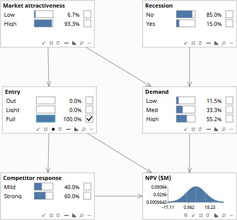
Rung 1 · seeing. Single-click Entry = Full (ordinary evidence). Attractiveness flows up to 93% High, the model infers it was a good market, and NPV reads +$6.5M. That upward flow is the confounding a dashboard books as real.
02The solution
The model should be a transparent map of how entry, spend, competitors and demand drive profit, assembled from your team’s knowledge and your data, not a black box. The same map answers all three questions strategy needs: why a result happened, what a move would do, and what would have happened under a different call.
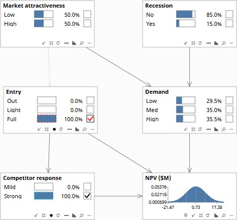
To show what one such map can do, we’ll build a deliberately simple model of a single decision, whether to enter a new regional market, and how hard. The lever has three settings (stay out, a light-touch pilot, or a full launch) and the outcome is two-year NPV. Six variables drive it: Market attractiveness, the chance of recession, the Entry decision, Demand, Competitor response, and the NPV they produce.
The solution was to model the relationships between the variables that drive profitability, and to be explicit about which variables cause which. We recognised, for example, that market demand is not a neutral backdrop, it is influenced by competitor activity and by prior investment in the market, which means observing high demand tells you something about what those upstream variables look like. Sunk costs and execution environment both influence outcomes but through different mechanisms: one affects the decision itself, the other shapes how that decision plays out. When you observe a variable in this model, you are effectively filtering the data to cases where that variable takes a particular value, and that filter ripples through the model, shifting related variables up and down accordingly. When you intervene on a variable, forcing it to a value regardless of what caused it, you break that ripple effect and get a cleaner answer: not what markets that look like this tend to produce, but what would happen if this specific decision were made When you abduct, you extract a particular case from the averages, locking in its idiosyncratic circumstances before asking what would have happened if one or more things had been different.
03What the solution answers
Instead of one forecast, our model will play out each option as a range of outcomes.
- A full launch has the best expected profit but a real chance of a loss if competitors retaliate.
- A light pilot earns less on average but rarely loses money.
- Staying out will get us zero.
Which to pick depends on the board’s appetite for risk, and the model puts that trade-off on the table instead of burying it inside an average.
| Option (do) | Expected NPV | Chance of a loss |
|---|---|---|
| Full launch | +$3.3M | 44% |
| Light pilot | +$2.5M | 16% |
| Stay out | $0 | , |
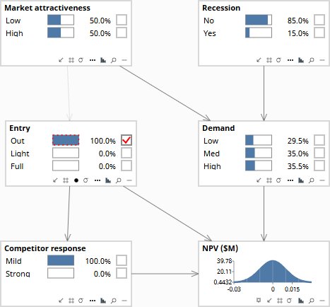
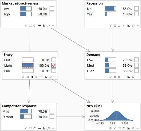
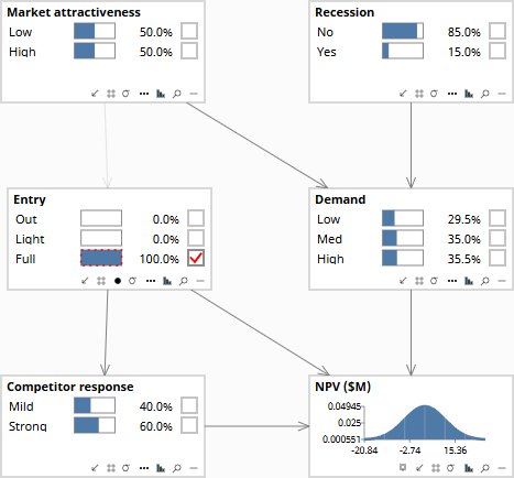
Two uses, one before acting, one after.
- Before: a counterfactual pre-mortem: “would the full launch still avoid a loss if a recession hit demand?” The chance of a loss climbs to roughly two in three, so you build contingencies into the plan.
- After: honest attribution: we went full and lost $3M. The model reconstructs what happened, then re-runs that same recovered world under a smaller move, a $1.8M loss. So the aggressive call cost about $1.2M in the world that occurred: a lesson for the next market, not a write-off blamed on luck.
The same model that planned the entry now runs it. As quarterly results arrive, share captured, competitor pricing, you feed them in and the forecast updates itself. When the first quarter comes in soft, the chance of a loss climbs from a little under half to three in five, which trips the pull-back trigger you agreed in advance. Plan, act, observe, update, re-decide: on one living model, not a slide deck that is stale the day it ships.
Every number carries honest confidence rather than false precision. The model shows which one or two assumptions swing the decision, so you spend your diligence there and nowhere else. And because it is your team’s reasoning written down, it is auditable and defensible: to a board, an investment committee, or a regulator, not a score no one can explain.
04 Inside the Model
A language model can speak fluently about any domain. It cannot know one. The .bayes file is the knowledge the LLM is missing: a causal map of the domain, auditable, versioned, and wrong in specific correctable ways.
Optionally open EnteringAMarket.bayes in Bayes Server or any equivalent tool. The model is the thing; the software that runs it is a commodity. The model is the thing; the software that runs it is a commodity.
Two gestures, one reading
- Observe (Rung 1), single-click a state; it goes to 100% and information flows up to parents.
- Do / intervene (Rung 2–3), right-click the node → Do(state), or hold Shift and click the state. A red checkmark appears on the state and incoming links dim; parents stay at their priors.
- Read NPV: keep NPV ($M) queried; its mean shows on the monitor, and the chance of a loss is the density mass left of $0.
- Clear all evidence between rungs (Edit Evidence → clear, or select nodes + Delete).
Rung 1: seeing
- Clear evidence.
- Observe Entry = Full (single-click, not Shift).
- You should see NPV +$6.5M, Market attractiveness jump to ~93% High, loss ~28%. The upward flow to attractiveness is the confounding.
Rung 2: doing (clear between each)
- Right-click Entry → Do(Out) → NPV $0.
- Do(Light) → +$2.5M, loss ~16%.
- Do(Full) → +$3.3M, loss ~44%. Note the red checkmark and attractiveness holding at 50/50.
- Pre-mortem: with Do(Full) still set, also observe Recession = Yes → −$0.9M, loss ~66%.
Rung 3: counterfactual attribution
Optionally open EnteringAMarket_CF.bayes, abduct the realized world by observing the actuals, re-observe the recovered U’s, then Do(Light) and read NPV.
Summary: every configuration and its reading
| Configuration | NPV | Loss | On screen |
|---|---|---|---|
| Observe Entry = Full (Rung 1) | +$6.5M | ~28% | Attractiveness → 93% High |
| Do(Out) | $0 | , | red checkmark; Attr 50/50 |
| Do(Light) | +$2.5M | ~16% | Competitor 70 / 30 |
| Do(Full) | +$3.3M | ~44% | Competitor 40 / 60 |
| Do(Full) + observe Recession = Yes | −$0.9M | ~66% | pre-mortem |
| Observe Full, Med, Strong | −$3.0M | , | the realized world |
| Do(Light) on abducted U’s | −$1.8M | , | genuine counterfactual |
| Do(Full) + observe Competitor = Strong | +$0.7M | ~60% | execution update |
05 Just Ask
The model is a file, not a locked tool. Any capable LLM can load the model’s XML and reason over it, so anyone on the team can interrogate the strategy in plain English and still get answers that keep seeing, doing and imagining apart.
do(light) → +$2.5M, ~1-in-6 chance of a loss
do(full) → +$3.3M, but ~4-in-9 chance of a loss
Same model, same three rungs, just driven in conversation. No one had to open Bayes Server to get a Rung-2 decision or a Rung-3 attribution.
- Timing sensitivity. Would delaying entry by two quarters change the expected value ranking?
- Competitive response. How does the expected value shift if a competitor enters first?
- Real options. What is the value of waiting for one more data point before committing?
- Portfolio view. Does this entry decision cannibalize expected value from an existing market?
- Exit conditions. At what point would the model recommend reversing the decision?
06 The Engagement
Elicit the structure from the people who know how the business actually works, parameterise it from your data and their judgment, validate it against what you can, and hand over a strategy simulator your team runs every planning cycle: and keeps feeding as the strategy plays out.
Sources: Pearl, J., 2009, Causality: Models, Reasoning, and Inference (2nd ed.), Cambridge University Press · Pearl, J. & Mackenzie, D., 2018, The Book of Why, Basic Books · Howard, R. & Matheson, J., 2005, “Influence Diagrams,” Decision Analysis 2(3). Figures on this page are computed from the accompanying model, EnteringAMarket.bayes.
The Deeper Trade
The model does not replace the expert who built it. It frees her from being the bottleneck for every routine version of this question, so she can spend her judgment on the cases that actually need it, and keep making the model better.
Tool-agnostic by design, the model is the asset; the environment follows the engagement.