Manufacturing

01 The Decision

A PRECISION COMPONENTS MANUFACTURER is running at 2.3% defect rate, above the 1.5% contractual threshold on a high-value aerospace account. The operations team has five candidate causes: material batch variation, machine calibration drift, operator technique, ambient temperature, and tooling wear. All five correlate with defect rates in the historical data. All five are expensive to address. The question is which one to address first.

The standard approach: regression of defect rate on all five, produces coefficients for each candidate. It does not answer which intervention most reduces the defect rate, because it cannot distinguish causes from confounders. Tool wear and machine calibration both correlate with defect rate. But tool wear may cause machine calibration drift, not the other way around. Addressing calibration without addressing tool wear treats the symptom.

02 The solution

The causal graph, elicited from the process engineers and quality team, encodes three pathways from upstream variables to defect rate:

OperatorTechnique moderates pathway 2, skilled operators detect and correct calibration drift earlier. It does not cause defects directly. Controlling for it in a regression attenuates the apparent effect of calibration drift without addressing the root cause.

The solution was to model the relationships between the variables that drive defect rates, and to be explicit about which variables cause which. We recognised, for example, that calibration drift is not a root cause, it is a symptom of tooling wear. Addressing calibration directly without addressing the upstream tooling condition treats the symptom, and the drift returns within production cycles. Material batch variation and ambient temperature both influence dimensional tolerance, which means they are confounders of each other in regression: a model that includes both without encoding their separate pathways will misattribute the effect of one to the other. When you observe a variable in this model, you are effectively filtering the data to cases where that variable takes a particular value, and that filter ripples through the model, shifting related variables up and down accordingly. When you intervene on a variable, forcing it to a value regardless of what caused it, you break that ripple effect and get a cleaner answer: not what production runs that look like this tend to produce, but what would happen if this specific upstream condition were corrected When you abduct, you extract a particular case from the averages, locking in its idiosyncratic circumstances before asking what would have happened if one or more things had been different.

03 What the solution answers

do(ToolingWear = Reduced 40%) vs do(MaterialBatch = Tightened) vs do(CalibrationDrift = Corrected). Each severs the node’s incoming edges and reads the downstream effect on DefectRate.

The tooling replacement schedule was delayed 3 weeks due to a supply chain disruption. 847 components were produced in this window. Would the contractual breach have occurred under the original schedule?

04 Inside the Model

A language model can speak fluently about any domain. It cannot know one. The .bayes file is the knowledge the LLM is missing: a causal map of the domain, auditable, versioned, and wrong in specific correctable ways.

Rung 1, Diagnostic: which upstream state is most consistent with this defect pattern?

Prior obs(DefectRate = 1.5) + obs(SurfaceFinish = 1.2)

Prior, no evidence set

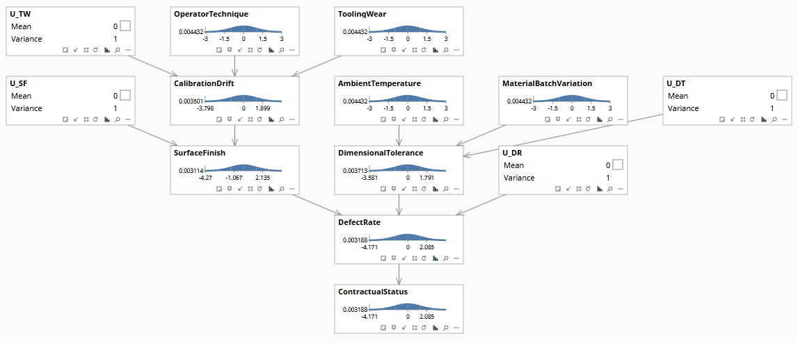
Baseline before any query. All nodes at prior distributions. DefectRate at population baseline.

Rung 2, Intervention: which fix has the most leverage?

do(ToolingWear = −40%) do(MaterialBatch = Tightened) do(CalibrationDrift = Corrected)

do(ToolingWear = −40%), optimal intervention

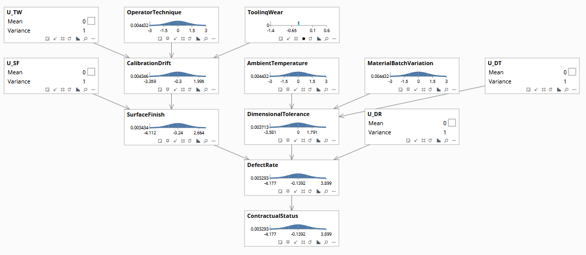
Tooling wear reduction severs the upstream driver of CalibrationDrift. DefectRate drops 1.1pp, below the 1.5% contractual threshold.

Rung 3, Counterfactual: did the tooling delay cause the contractual breach?

Step 1, Abduction Step 2, do(Tooling = OnSchedule)

Step 1, Abduction: breach period conditions entered

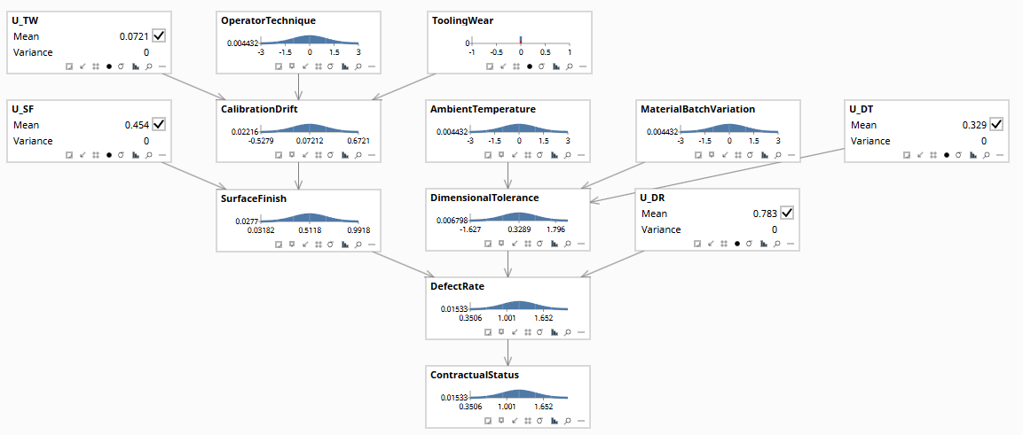
Actual tooling condition from the delay period entered as evidence. U nodes anchored to this specific production window. Ready for counterfactual.

05 Just Ask

The model is a file. Any capable LLM can load its XML and answer quality attribution questions in plain English.

Same model, three rungs. The audit trail is the .bayes file, not the regression output.

06 The Engagement

Elicit the causal structure from your process engineers, they already know that tool wear causes calibration drift, not the other way around. Encode that knowledge as a graph. Parameterize it from your production data. The result is a model that tells you which intervention to make, how much it will reduce the defect rate, and whether a specific batch failure was caused by a supplier event or a process failure.

• Intervention prioritisation. Which upstream variable to address first, not the one with the highest regression coefficient, but the one with the most causal leverage.
• Contractual attribution. When a supplier disruption coincides with a quality breach, the model separates how much of the breach was caused by the disruption vs process failure, the number your legal team needs.
• Ongoing monitoring. The same model runs diagnostics in production: given this defect pattern, which upstream state is most likely, and where should inspection be directed?

This case study is a composite drawn from published manufacturing quality and process engineering literature. Specific figures are representative. No individual organisation or engagement is described.