Scenarios
Executive TechnicalRather than change evidence by hand one assumption at a time, name the worlds you care about, stable burn with intact filter, stable burn with industrial waste, store each as a set of evidence, and compare what your model says across all of them at once.
This Example
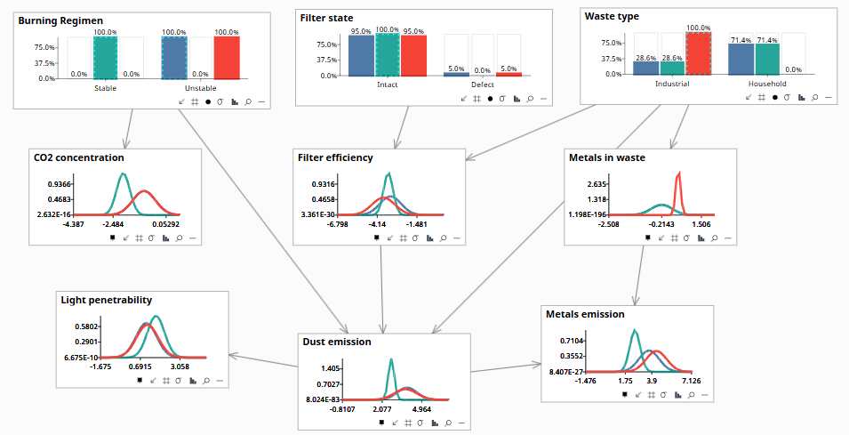
A waste incineration model with three scenarios, unstable combustion baseline (blue), stable burn with intact filter (teal), stable burn with industrial waste (red), showing how emissions, filter efficiency, and light penetrability shift across all three worlds simultaneously.
01 The Gap
Three operating conditions. One model. What do the outcomes look like across all three?
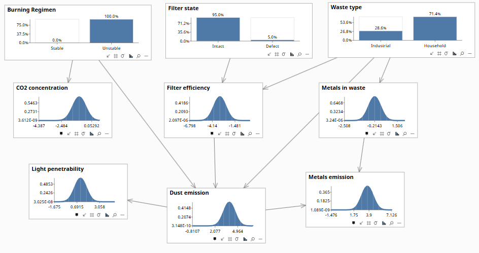
An environmental compliance officer needs to understand how emissions vary across three operating conditions at a waste incineration plant: the baseline prior, stable combustion with an intact filter, and stable combustion processing industrial waste. The network has nine nodes, burning regimen, filter state, and waste type as root causes; CO2 concentration, filter efficiency, and metals in waste as intermediate variables; dust emission, metals emission, and light penetrability as downstream outcomes.
The conventional approach is to set each combination of evidence by hand, read off the posteriors, reset, and try to hold all three sets of distributions in memory for comparison. Three worlds, nine nodes, twenty-seven distributions. That comparison cannot be done reliably by hand, and it does not force anyone to commit to what the worlds are before the analysis begins.
02 The component
Evidence bundles, named, reusable worlds the model runs in parallel.
The scenarios component bundles evidence into named, reusable worlds. For the waste model: Unstable combustion (blue, Burning Regimen = Unstable) is world A; Stable burn, intact filter (teal, Burning Regimen = Stable + Filter state = Intact) is world B; Stable burn, industrial waste (red, Burning Regimen = Stable + Waste type = Industrial) is world C. Run all three against Waste.bayes and what comes back is a side-by-side comparison of all nine node distributions simultaneously, the causal structure held constant across every world.
A scenario is a saved world. Name the world, bind the evidence, run the model, store the result. The comparison, not any single posterior, is the product. Scenario analysis does something prior to optimization: it lays out how the world could differ and what each difference would mean, without collapsing to one recommendation.
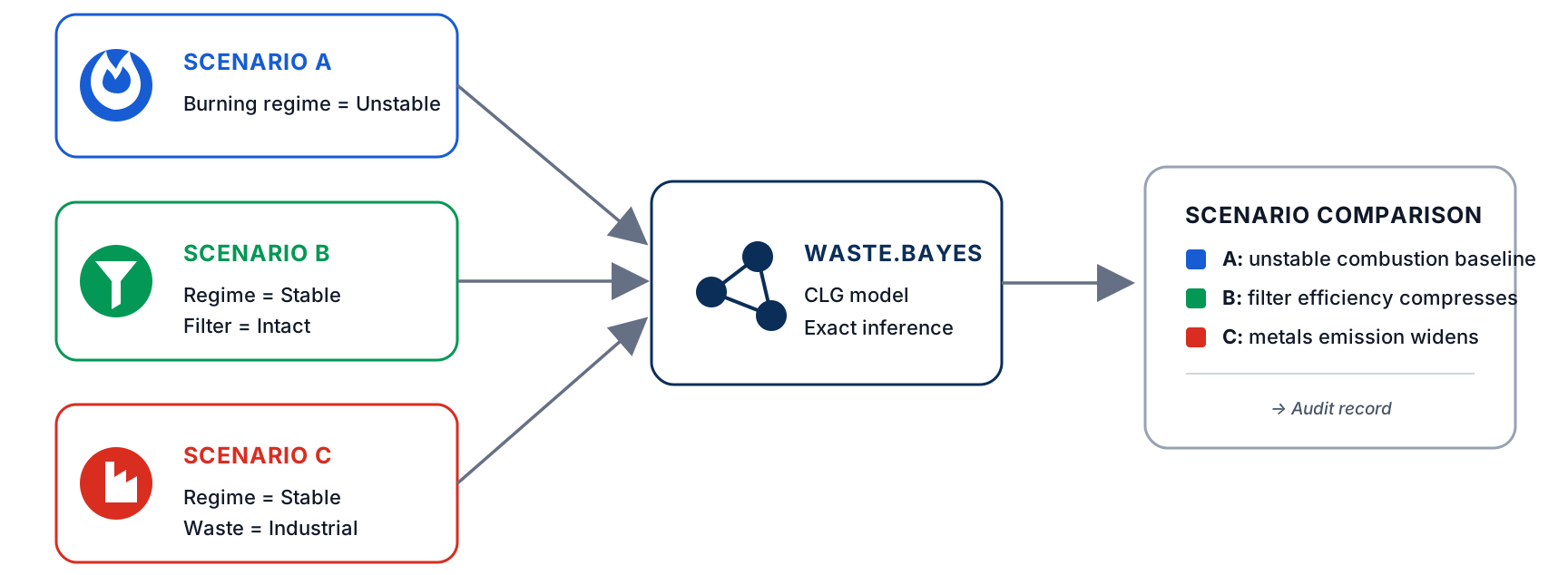
In Bayes Server's implementation, a scenario is evidence plus a name, a color for visualization, and an optional description. Scenarios can be saved, loaded, and reused, the world definitions persist alongside the model.
Visual overlay shows the direction of shift. Information-theoretic measures quantify it. Bayes Server's Jensen-Shannon Divergence and Kullback-Leibler Divergence calculators accept two scenarios as inputs and return a scalar distance between their posterior distributions on any target node.
| Field | What it holds |
|---|---|
| Scenario | A named world, e.g. "Prior," "Stable + Intact," "Stable + Industrial", defined by which evidence is set in it |
| Compared outcomes | The specific outcomes checked across every scenario, side by side |
| Results | Each scenario's distribution over each compared outcome, the same questions, answered under every world at once |
Scenarios is distinct from Optimization (10): scenarios lay out the landscape; optimization searches it. You reach for scenarios when the futures are exogenous, you do not choose what waste type arrives at the plant, and for optimization when the levers are yours to pull.
03 How it works
Three worlds defined. Three passes. Nine distributions compared.
IN THIS EXAMPLE, THREE WORLDS ARE DEFINED AS EVIDENCE BUNDLES. The model runs each in turn. All nine node distributions appear simultaneously, emissions, filter efficiency, CO2 concentration, light penetrability, across every world. Nothing is toggled by hand; nothing is held in memory.
Define. Scenario A (blue): Burning Regimen = Unstable, the worst-case combustion baseline. Scenario B (teal): Burning Regimen = Stable, Filter state = Intact. Scenario C (red): Burning Regimen = Stable, Waste type = Industrial. Each world is named, colored, and saved.
Run. The model evaluates each scenario in turn, computing the posterior over all nine nodes. Scenario B tightens the filter efficiency distribution and compresses dust emission. Scenario C shifts metals in waste sharply right and widens metals emission. The computation is exact; each scenario is independent.
Compare. The three distributions appear side by side on every node. The shape of the compliance question becomes legible: intact filter shifts emissions left; industrial waste shifts metals right. The contrast between B and C is what the compliance report needs, and it is produced without touching the model.
A scenario can combine any number of evidence bindings. A worst-case world, unstable combustion, defective filter, industrial waste, is three bindings in one scenario, compared against the baseline in a single run.
04 The Brains
The model evaluating multiple futures simultaneously.
Scenario analysis is the brains evaluating multiple futures simultaneously, something that requires an explicit domain model, because an implicit one cannot hold multiple named worlds in structured comparison.
The Waste.bayes model below is the domain model for this example. Load it in Bayes Server, open the accompanying Waste.scenarios file, and the three-scenario comparison in the screenshot above reproduces exactly.
| Scenario | Defined by |
|---|---|
| Prior | No evidence set, the baseline world |
| Stable + Intact | Burning Regimen = Stable, Filter State = Intact |
| Stable + Industrial | Burning Regimen = Stable, Waste Type = Industrial |
05 Query in plain English
What do the outcomes look like across our three operating worlds?
Scenarios answers the question before the decision: what do the emissions look like across our three operating worlds?
The audit trail is the ScenarioComparison. The scenario definitions, every evidence binding in every world, are part of the audit trail.
06 Where it sits
First Action component, between the epistemic cluster and Optimization.
Scenarios is the first Cognitive Primitives, Action component. It sits between the epistemic cluster (05–08, which asks whether the current model is trustworthy) and Optimization (10, which searches for the best action). Scenarios is the bridge: it maps out the action landscape before the optimizer searches it.
Upstream: the domain model and the named worlds defined by the analyst, in the waste case, the compliance officer's two operating modes. Downstream: the ScenarioComparison feeds Optimization (10), which searches for the best action given the landscape the scenarios revealed, whether to require enhanced filter maintenance for industrial loads. It also feeds 12 BPMN Integration directly when the comparison is the output, such as a compliance report showing emission distributions across named operating modes.
For a full three-rung treatment of a single claim, diagnostic inference, causal intervention, and individual counterfactual, see the Insurance Attribution Walkthrough →